5  OpenStreetMap

This session is all about OpenStreetMap. The following will resources provide an overview of the OpenStreetMap project:

• A clip

• This piece is about how OpenStreetMap is currently being created and some of the implications this may have.
• Anderson et al. (Anderson, Sarkar, and Palen 2019) provide some of the academic underpinnings to the views expressed in the above piece.

5.1 Packages and modules

import geopandas
import contextily
import matplotlib.pyplot as plt
from IPython.display import GeoJSON

5.2 Data

Since some of the query options we will discuss involve pre-defined extents, we will read the Madrid neighbourhoods dataset first.

Assuming you have the file locally on the path ../data/:

neis = geopandas.read_file("../data/neighbourhoods.geojson")

To make some of the examples below computationally easier on OpenStreetMap servers, we will single out the smallest neighborhood:

areas = neis.to_crs(
    epsg=32630
).area

smallest = neis[areas == areas.min()]
smallest

	neighbourhood	neighbourhood_group	geometry
98	Atalaya	Ciudad Lineal	MULTIPOLYGON (((-3.66195 40.46338, -3.66364 40...

fig, ax = plt.subplots()

smallest.plot(
    facecolor="none", edgecolor="blue", linewidth=2, ax=ax
)

contextily.add_basemap(
    ax, 
    crs=smallest.crs, 
    source=contextily.providers.OpenStreetMap.Mapnik
)

plt.show()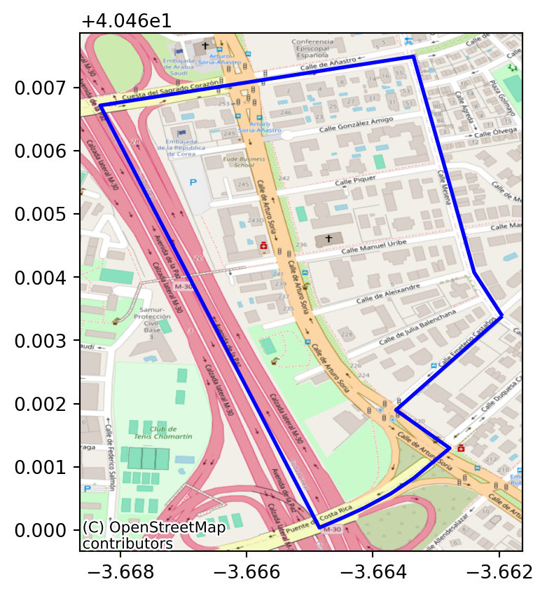

5.3 osmnx

Let’s import one more package, osmnx, designed to easily download, model, analyse, and visualise street networks and other geospatial features from OpenStreetMap.

import osmnx as ox

Here is a trick (courtesy of Martin Fleischmann to pin all your queries to OpenStreetMap to a specific date, so results are always reproducible, even if the map changes in the meantime.

ox.settings.overpass_settings = (
    '[out:json][timeout:90][date:"2021-03-07T00:00:00Z"]'
)

Note

Much of the methods covered here rely on the osmnx.features module. Check out its reference here.

There are two broad areas to keep in mind when querying data on OpenStreetMap through osmnx:

• The interface to specify the extent of the search.

• The nature of the entities being queried. Here, the interface relies entirely on OpenStreetMap’s tagging system. Given the distributed nature of the project, this is variable, but a good place to start is:

https://wiki.openstreetmap.org/wiki/Tags

Generally, the interface we will follow involves the following:

received_entities = ox.features_from_XXX(
    <extent>, tags={<key>: True/<value(s)>}, ...
)

The <extent> can take several forms. We can print out the available forms:

[i for i in dir(ox) if "features_from_" in i]

['features_from_address',
 'features_from_bbox',
 'features_from_place',
 'features_from_point',
 'features_from_polygon',
 'features_from_xml']

The tags follow the official feature spec.

5.4 Buildings

blgs = ox.features_from_polygon(
    smallest.squeeze().geometry, tags={"building": True}
)

fig, ax = plt.subplots()

blgs.plot(ax=ax)

plt.show()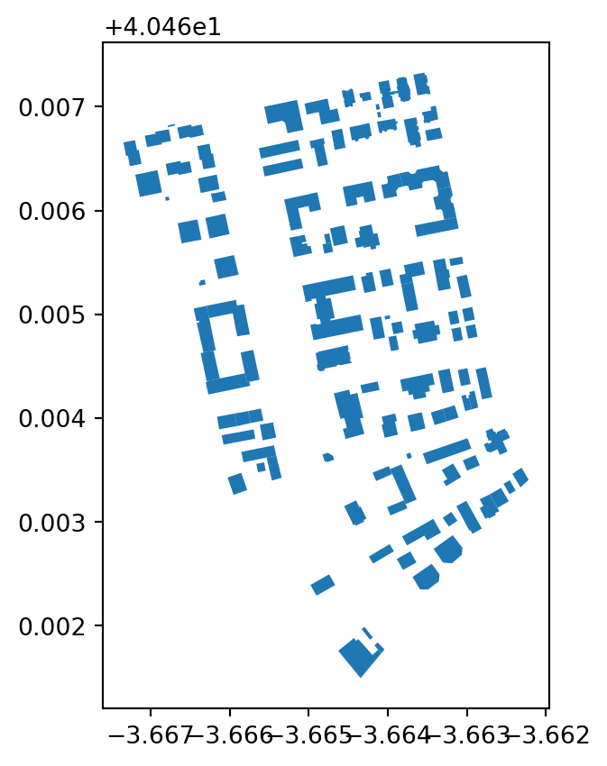

blgs.info()

<class 'geopandas.geodataframe.GeoDataFrame'>
MultiIndex: 115 entries, ('way', 442595762) to ('way', 577690922)
Data columns (total 27 columns):
 #   Column            Non-Null Count  Dtype   
---  ------            --------------  -----   
 0   name              2 non-null      object  
 1   amenity           2 non-null      object  
 2   geometry          115 non-null    geometry
 3   nodes             115 non-null    object  
 4   building          115 non-null    object  
 5   addr:housenumber  21 non-null     object  
 6   addr:postcode     3 non-null      object  
 7   addr:street       9 non-null      object  
 8   denomination      1 non-null      object  
 9   phone             2 non-null      object  
 10  religion          1 non-null      object  
 11  source            1 non-null      object  
 12  source:date       1 non-null      object  
 13  url               1 non-null      object  
 14  wheelchair        1 non-null      object  
 15  building:levels   11 non-null     object  
 16  addr:city         8 non-null      object  
 17  addr:country      6 non-null      object  
 18  wikidata          1 non-null      object  
 19  website           1 non-null      object  
 20  country           1 non-null      object  
 21  diplomatic        1 non-null      object  
 22  name:en           1 non-null      object  
 23  name:fr           1 non-null      object  
 24  name:ko           1 non-null      object  
 25  office            1 non-null      object  
 26  target            1 non-null      object  
dtypes: geometry(1), object(26)
memory usage: 29.7+ KB

blgs.head()

		name	amenity	geometry	nodes	building	addr:housenumber	addr:postcode	addr:street	denomination	phone	...	addr:country	wikidata	website	country	diplomatic	name:en	name:fr	name:ko	office	target
element_type	osmid
way	442595762	NaN	NaN	POLYGON ((-3.66377 40.46317, -3.66363 40.46322...	[4402722774, 4402722775, 4402722776, 440272277...	yes	NaN	NaN	NaN	NaN	NaN	...	NaN	NaN	NaN	NaN	NaN	NaN	NaN	NaN	NaN	NaN
	442595763	NaN	NaN	POLYGON ((-3.66394 40.46346, -3.66415 40.46339...	[4402722778, 4402722779, 4402722780, 440272278...	yes	NaN	NaN	NaN	NaN	NaN	...	NaN	NaN	NaN	NaN	NaN	NaN	NaN	NaN	NaN	NaN
	442595764	NaN	NaN	POLYGON ((-3.66379 40.46321, -3.66401 40.46314...	[4402722782, 4402722783, 4402722784, 440272278...	yes	NaN	NaN	NaN	NaN	NaN	...	NaN	NaN	NaN	NaN	NaN	NaN	NaN	NaN	NaN	NaN
	442595765	NaN	NaN	POLYGON ((-3.66351 40.46356, -3.66294 40.46371...	[4402722786, 4402722787, 4402722788, 440272278...	yes	NaN	NaN	NaN	NaN	NaN	...	NaN	NaN	NaN	NaN	NaN	NaN	NaN	NaN	NaN	NaN
	442596830	NaN	NaN	POLYGON ((-3.66293 40.46289, -3.66281 40.46294...	[4402729658, 4402729659, 4402729660, 440272966...	yes	NaN	NaN	NaN	NaN	NaN	...	NaN	NaN	NaN	NaN	NaN	NaN	NaN	NaN	NaN	NaN

5 rows × 27 columns

If you want to visit the entity online, you can do so at:

https://www.openstreetmap.org/<unique_id>

Note

Challenge: Extract the building footprints for the Sol neighbourhood in neis.

5.5 Other polygons

park = ox.features_from_place(
    "Parque El Retiro, Madrid", tags={"leisure": "park"}
)

fig, ax = plt.subplots()

park.plot(
    facecolor="none", edgecolor="blue", linewidth=2, ax=ax
)

contextily.add_basemap(
    ax, 
    crs=smallest.crs, 
    source=contextily.providers.OpenStreetMap.Mapnik
)

plt.show()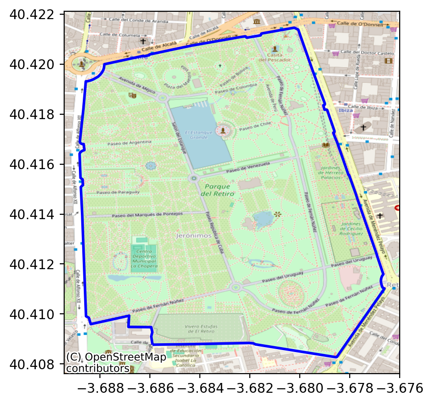

5.6 Points of interest

Bars around Atocha station:

bars = ox.features_from_address(
    "Puerta de Atocha, Madrid", tags={"amenity": "bar"}, dist=1500
)

We can quickly explore with GeoJSON:

bars.explore()

Make this Notebook Trusted to load map: File -> Trust Notebook

And stores within Malasaña:

shops = ox.features_from_address(
    "Malasaña, Madrid, Spain", # Boundary to search within
    tags={
        "shop": True,
        "landuse": ["retail", "commercial"],
        "building": "retail"
    },
    dist=1000
)

shops.explore()

Make this Notebook Trusted to load map: File -> Trust Notebook

We use features_from_place for delineated areas (“polygonal entities”):

cs = ox.features_from_place(
    "Madrid, Spain",
    tags={"amenity": "charging_station"}
)

cs.explore()

Make this Notebook Trusted to load map: File -> Trust Notebook

Similarly, we can work with location data. For example, searches around a given point:

bakeries = ox.features_from_point(
    (40.418881103417675, -3.6920446157455444),
    tags={"shop": "bakery", "craft": "bakery"},
    dist=500
)

bakeries.explore()

Make this Notebook Trusted to load map: File -> Trust Notebook

Note

Challenge:

• How many music shops does OSM record within 750 metres of Puerta de Alcalá?

- Are there more restaurants or clothing shops within the polygon that represents the Pacífico neighbourhood in neis table?

5.7 Streets

Street data can be obtained as another type of entity, as above; or as a graph object.

5.7.1 Geo-tables

centro = ox.features_from_polygon(
    neis.query("neighbourhood == 'Sol'").squeeze().geometry,
    tags={"highway": True}
)

We can get a quick peak into what is returned (in grey), compared to the region we used for the query:

fig, ax = plt.subplots()

neis.query(
    "neighbourhood == 'Sol'"
).plot(color="k", ax=ax)

centro.plot(
    ax=ax, 
    color="0.5", 
    linewidth=0.2, 
    markersize=0.5
)

plt.show()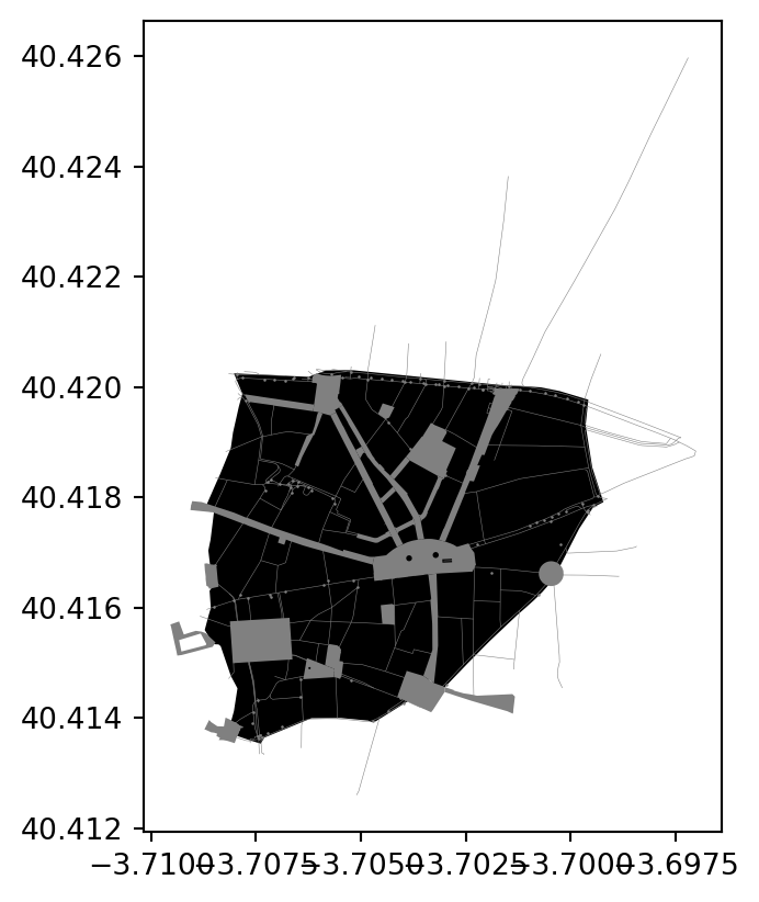

This however will return all sorts of things:

centro.geometry

element_type  osmid    
node          21734214                             POINT (-3.70427 40.41662)
              21734250                             POINT (-3.70802 40.41612)
              21734252                             POINT (-3.70847 40.41677)
              21968134                             POINT (-3.69945 40.41786)
              21968197                             POINT (-3.70054 40.41645)
                                                 ...                        
way           907553665    LINESTRING (-3.70686 40.41380, -3.70719 40.41369)
              909056211    LINESTRING (-3.70705 40.42021, -3.70680 40.42020)
relation      5662178      POLYGON ((-3.70948 40.41551, -3.70952 40.41563...
              7424032      POLYGON ((-3.70263 40.41712, -3.70253 40.41714...
              8765884      POLYGON ((-3.70636 40.41475, -3.70635 40.41481...
Name: geometry, Length: 609, dtype: geometry

5.7.2 Spatial graphs

The graph_from_XXX() functions return clean, processed graph objects for the street network. Available options are:

[i for i in dir(ox) if "graph_from_" in i]

['graph_from_address',
 'graph_from_bbox',
 'graph_from_gdfs',
 'graph_from_place',
 'graph_from_point',
 'graph_from_polygon',
 'graph_from_xml']

Here is an example:

centro_gr = ox.graph_from_polygon(
    neis.query("neighbourhood == 'Sol'").squeeze().geometry,
)

This is indeed a graph object (as defined by the networkx package):

centro_gr

<networkx.classes.multidigraph.MultiDiGraph at 0x153a19810>

To visualise it, there are several plotting options:

[i for i in dir(ox) if "plot_graph" in i]

['plot_graph', 'plot_graph_folium', 'plot_graph_route', 'plot_graph_routes']

For example:

ox.plot_figure_ground(centro_gr)
plt.show()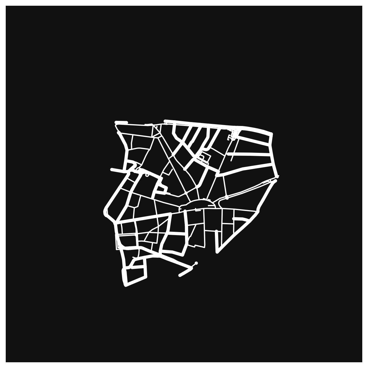

ox.graph_to_gdfs(centro_gr, nodes=False).explore()

Make this Notebook Trusted to load map: File -> Trust Notebook

Note

Challenge: How many bookshops are within a 50m radious of the Paseo de la Castellana?

This one involves the following steps:

• Extracting the street segment for Paseo de la Castellana
• Drawing a 50m buffer around it
• Querying OSM for bookshops

5.8 Next steps

If you found the content in this block useful, the following resources represent some suggestions on where to go next:

• Parts of the block are inspired and informed by Geoff Boeing’s excellent course on Urban Data Science
• More in depth content about osmnx is available in the official examples collection
• Boeing (2020) {cite}boeing2020exploring illustrates how OpenStreetMap can be used to analyse urban form (Open Access)

Anderson, Jennings, Dipto Sarkar, and Leysia Palen. 2019. “Corporate Editors in the Evolving Landscape of OpenStreetMap.” ISPRS International Journal of Geo-Information 8 (5): 232.